Radmap: visualizing molecular reactivity with isodistance potential energy surfaces

• Read the paper
• View the code on GitHub

When a free radical meets a molecule, where does it attack? For benzene the answer is obvious, because every carbon is the same. For azulene, pyrene or a new ligand nobody has made before, it isn’t, and finding out in the lab takes time, material and sometimes a particle accelerator.

Radmap is a program I wrote as a chemistry student at Saint Mary’s University in Halifax, in the Atlantic Centre for Green Chemistry, to answer that question computationally. It shows the earliest moment of a reaction between a molecule and a single atom (a hydrogen atom, a proton, a hydride, a bromine atom or anything else monoatomic) as a colored surface wrapped around the molecule. Red marks the low-energy spots, where the incoming atom is drawn in and a radical is most likely to add.

We described the method in the Journal of Molecular Graphics and Modelling:

Andrew K. Long, Jason A. Fawcett, Jason A.C. Clyburne and Cory C. Pye. RADMAP: Simple probes for rapid assessment of complex reactivity: A method and case studies on the reaction of hydrogen atoms with unsaturated organic molecules. J. Mol. Graph. Model. 64, 147–152 (2016).

Why muons

The problem came from muon chemistry. A positive muon that captures an electron forms muonium, which behaves chemically like a hydrogen atom with about a ninth of the mass. Fire muons into a sample and the muonium adds to the molecules in it, just as a hydrogen atom would. In a transverse-field muon spin resonance (µSR) experiment, each distinct radical that forms gives its own pair of signals.

So before running an experiment you want to know how many places the muonium can add, and roughly how much of each adduct will form. That tells you how many signals to look for and how strong each should be. Beam time at a muon facility is scarce, and a good prediction makes it go further.

How it works

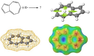Azulene + H·: the question, a probe atom moved over the molecule, the surface it samples, and the finished map.

Radmap works in four steps:

1. Build a surface. Starting from a structure loaded from a .mol file, Radmap draws a solvent-accessible surface around the molecule. Every point on it sits a fixed distance outside the atoms (by default a 1.2 Å probe radius beyond each atom’s van der Waals radius), which is what isodistance means here. A resolution setting controls how many points the mesh has.
2. Place the probe. For every point on the mesh, Radmap writes a Gaussian input file containing the molecule plus the probe atom at that point, and a batch file to run them all. You choose the probe, the charge and multiplicity, and the method and basis set. The default is a short two-step optimization at the unrestricted B3LYP/6-31G level, which suits an open-shell radical.
3. Compute. Gaussian runs every job. This is the slow part: one quantum chemistry calculation per point on the surface, which is why the batch file can be split across machines.
4. Paint. Radmap reads the energy out of each output file, smooths the values onto the displayed surface with a Gaussian-weighted average, and colors it from blue (high energy, where the probe is pushed away) to red (low energy, where the probe is drawn in).

The result is a potential energy surface that isn’t a flat slice through space but wraps the whole molecule, so every side of it can be compared at once. The red regions predict where addition happens. The relative energies of the red spots also give a qualitative estimate of how much of each adduct forms, which says something about the molecule’s kinetic stability as well as its reactivity.

The interface is built on Jmol, the open source molecular viewer, so the finished map can be rotated and inspected like any other Jmol model. Radmap itself is open source too.

Reading the maps

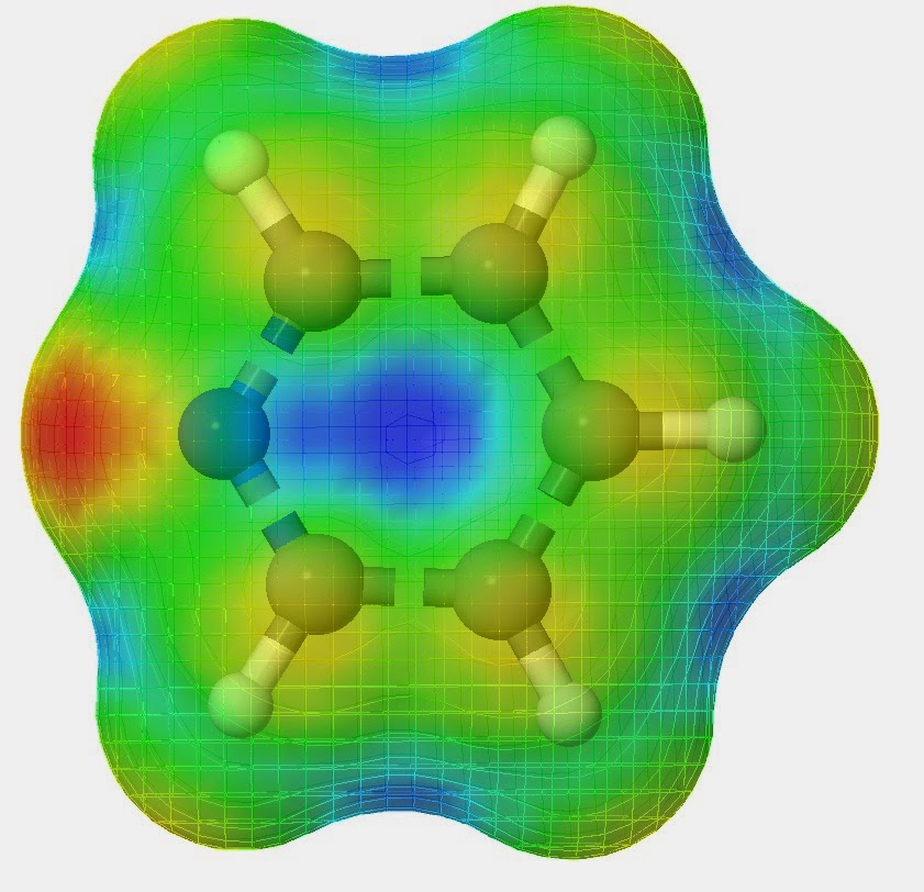
Pyridine + H·. The strongest red sits just outside the nitrogen, and the center of the ring is blue.

Pyridine is a good first example because it has only one feature that isn’t a C–H. The map picks it out straight away: the hot spot is at the nitrogen, and the ring carbons are all much cooler.

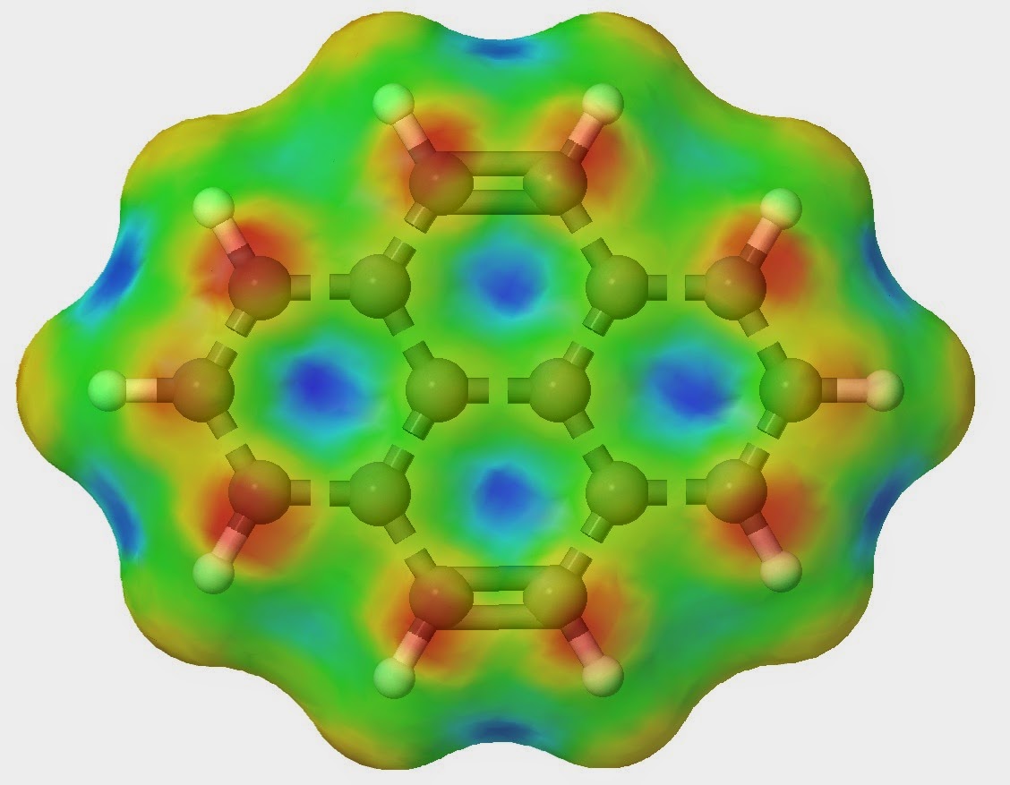Pyrene + H·. Red over the outer carbons, weaker at the 2 and 7 positions, and blue over the ring centers.

Pyrene is where the method starts to earn its keep. It has 10 C–H carbons, and the map separates them into groups: the carbons at the ends of the upper and lower double bonds and the carbons next to the ring junctions glow red, while the carbons in the middle of the left and right edges are noticeably cooler. Each distinct red site is a distinct radical, and a distinct µSR signal.

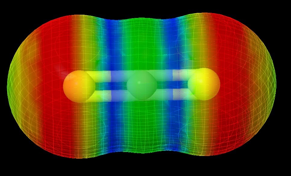Carbon disulfide + H·. The low-energy regions are the caps over the two sulfur atoms, not the carbon.

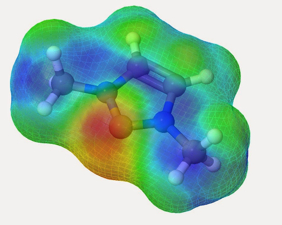1,3-Dimethylimidazol-2-ylidene, an N-heterocyclic carbene, + H·. The red patch is over the carbene carbon between the two nitrogens.

The carbene is a nice check. Earlier muonium experiments from the Clyburne group, with Paul Percival’s team, showed that the hydrogen atom adds to the carbene carbon, and that is exactly where Radmap puts the red.

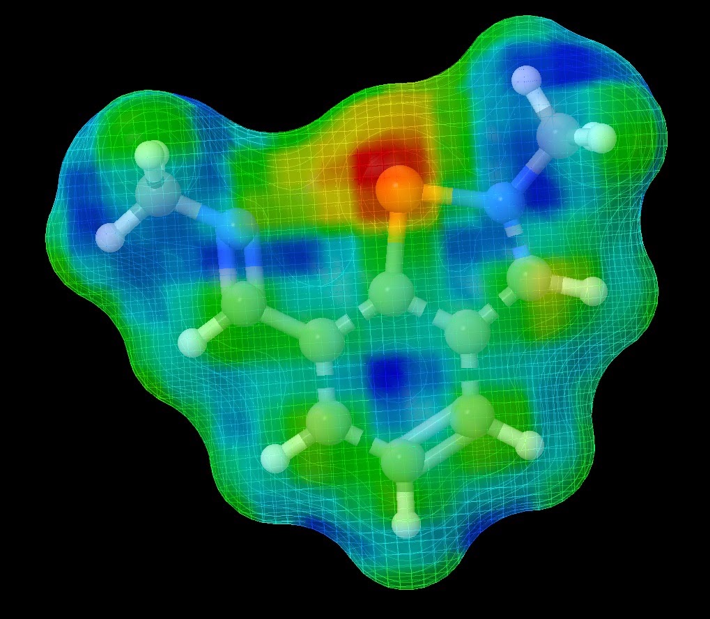A phosphorus pincer compound + H·. The reactive site is the phosphorus at the center.

This is also where Radmap is useful beyond muons. When you design a new ligand to bind to a metal, you want to know where its reactive sites are before you spend weeks making it. A Radmap surface, run with whichever probe fits the question, gives a quick first look.

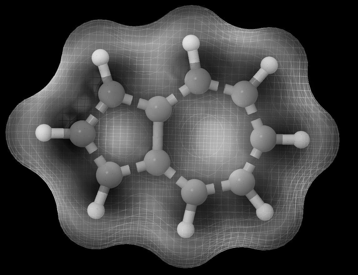Azulene, rendered in grayscale.

Limitations

Radmap is deliberately simple, and that has costs:

• It only sees the first contact. The probe is placed at a fixed distance and relaxed for only a couple of steps, so the map shows where an atom is drawn in, not the final product or the barrier to get there.
• It’s expensive. Every point on the mesh is a separate quantum chemistry job. A fine mesh on a large molecule means thousands of calculations.
• It’s qualitative. The colors rank sites against each other on one molecule. They aren’t rate constants, and the level of theory limits how far the numbers can be trusted.

Within those limits, it turns a question that used to need an experiment into a picture you can rotate on screen.

Credits

• Main developer: Andrew K. Long
• Advisers: Jason A.C. Clyburne and Cory C. Pye
• Co-author: Jason A. Fawcett
• Art design: Emily Rose

Thanks to Robert M. Hanson and everyone on the Jmol-Development mailing list for their help with this program, and to Jason Masuda for his input during development.