<?xml version="1.0" encoding="utf-8"?><feed xmlns="http://www.w3.org/2005/Atom" ><generator uri="https://jekyllrb.com/" version="3.10.0">Jekyll</generator><link href="https://www.andrewklong.com/feed.xml" rel="self" type="application/atom+xml" /><link href="https://www.andrewklong.com/" rel="alternate" type="text/html" /><updated>2026-10-01T08:34:57+00:00</updated><id>https://www.andrewklong.com/feed.xml</id><title type="html">Andrew Long</title><subtitle>I am a software developer and chemist</subtitle><entry><title type="html">Isle of Savreen: a tank of water you can tip</title><link href="https://www.andrewklong.com/blog/isle-of-savreen-a-tank-of-water-you-can-tip/" rel="alternate" type="text/html" title="Isle of Savreen: a tank of water you can tip" /><published>2026-10-01T00:00:00+00:00</published><updated>2026-10-01T00:00:00+00:00</updated><id>https://www.andrewklong.com/blog/isle-of-savreen-a-tank-of-water-you-can-tip</id><content type="html" xml:base="https://www.andrewklong.com/blog/isle-of-savreen-a-tank-of-water-you-can-tip/"><![CDATA[<ul class="actions special">
  <li><a href="/IsleOfSavreen/" class="button large">Launch Isle of Savreen</a></li>
  <li><a href="https://github.com/AndrewKL/IsleOfSavreen" class="button large">View the code on GitHub</a></li>
</ul>

<p><a href="/IsleOfSavreen/">Isle of Savreen</a> is the 3D follow-up to my
<a href="/blog/painting-water-with-the-navier-stokes-equations/">2D water simulator</a>:
a glass cube of water, a meter on a side, with a rusting fishing boat run
aground among mossy boulders inside. You look down on it like a model on a
table, and the arrows let you pick the tank up. Tip it and the water pours to
the low side and breaks over the rocks; jerk it sideways and it slams into the
far wall and climbs it. As in the 2D version, every bit of water is a brush
stroke, deep blue when slow and white foam when fast, and the sound is built
from the same physics.</p>

<h2 id="how-flip-turns-particles-into-water">How FLIP turns particles into water</h2>

<p>The water is about 7,500 particles, each a 2.5 cm drop that carries its own
position and velocity. Particles are good at being water: wherever there are
particles there’s water, everywhere else is air, so splashes, droplets and a
free surface come for free. What particles are bad at is the one rule water
lives by, that it can’t be squeezed. Checking that every bit of water has as
much flowing out as flowing in is easy on a grid and hard among scattered
points.</p>

<p>FLIP (Fluid-Implicit-Particle) uses both. The particles carry the water; a
coarse grid, 20 × 20 × 20 cells of 5 cm, enforces incompressibility. Brackbill
and Ruppel invented it for plasma physics in 1986, and Zhu and Bridson brought
it to graphics in 2005; it’s what film effects use for splashing water. Every
1/60 of a second, each step goes:</p>

<ol>
  <li><strong>Move the particles.</strong> Add gravity (and the tank’s forces, below), then
move each particle along its velocity. For a moment the water just flies.</li>
  <li><strong>Keep them spaced out.</strong> Anywhere two particles overlap, push them apart.
Without this they clump in some places and leave gaps in others.</li>
  <li><strong>Collide.</strong> Push any particle that ended up in a wall, the ship or a rock
back out to the surface, and stop it moving into it.</li>
  <li><strong>Particles to grid.</strong> Each particle spreads its velocity onto the eight
nearest cell faces, weighted by how close it is. The grid stores velocities
on cell faces rather than centers, so the flow through each face is exactly
what’s needed to count what enters and leaves each cell.</li>
  <li><strong>Make it incompressible.</strong> For every cell with water in it, add up the
flow out through its six faces. In real water that’s zero. Here it won’t
be, so nudge the faces until it is: push flow out of cells that are being
crammed and into ones that are draining. Each fix disturbs the neighbors,
so the grid is swept 40 times. That nudging is the pressure in the
Navier–Stokes equations. Cells packed with more particles than water at
rest would hold get an extra push outward, so the water doesn’t slowly
lose volume.</li>
  <li><strong>Grid back to particles.</strong> Each particle reads the corrected velocity
from the faces around it. Here’s the trick in the name: it doesn’t take
the grid’s velocity (that method, PIC, works but smears motion away and
the water turns to syrup); it keeps its own velocity and adds only the
<em>change</em> the grid made. That keeps all the small-scale motion the coarse
grid can’t represent. Pure FLIP is noisy, so the blend here is 90% FLIP
and 10% PIC, and that 10% stands in for water’s tiny viscosity.</li>
</ol>

<p>If the fastest water would move more than two cells in a step, the step is
split into smaller ones so nothing tunnels through a thin wall. In 3D each of
those stages touches three times as many neighbors as in 2D, which is why the
grid is coarser here, and why speed mattered (more below).</p>

<h2 id="moving-the-tank-without-moving-the-water">Moving the tank without moving the water</h2>

<p>The obvious way to tip a tank is to tip the grid. That’s the hard way: the
walls would cut diagonally through the cells. So the simulation never moves.
It runs in the tank’s own frame, where the walls and rocks always line up with
the grid, and moving the tank becomes forces the water feels, the ones you
feel in a car or on a roundabout:</p>

<ul>
  <li><strong>Tilt</strong> turns gravity: seen from inside the tank, “down” points at a
different wall.</li>
  <li><strong>Sliding</strong> pushes the water back, the way coffee sloshes when you start
walking.</li>
  <li><strong>Turning</strong> adds an outward push (centrifugal), a sideways drift of anything
moving (Coriolis), and a jolt as a turn starts and stops.</li>
</ul>

<p>Each arrow press is a short, smooth move that starts and ends at rest, so
these forces are known exactly. I checked them against textbook answers: a
tank accelerating sideways tilts its water surface to a slope of a/g, a tank
turned on its side ends with its water against the new floor, and water in a
spinning tank rises up the walls into a curved bowl.</p>

<p>A glowing light in the sky adds one more force. It swings from far left to
far right and back every 2.5 seconds, pulling the water toward it with about a
third the strength of gravity. A wave takes about 1.25 seconds to cross this
tank and back, so the light keeps the water sloshing without the motion
building up out of control.</p>

<h2 id="a-shipwreck-and-some-rocks">A shipwreck and some rocks</h2>

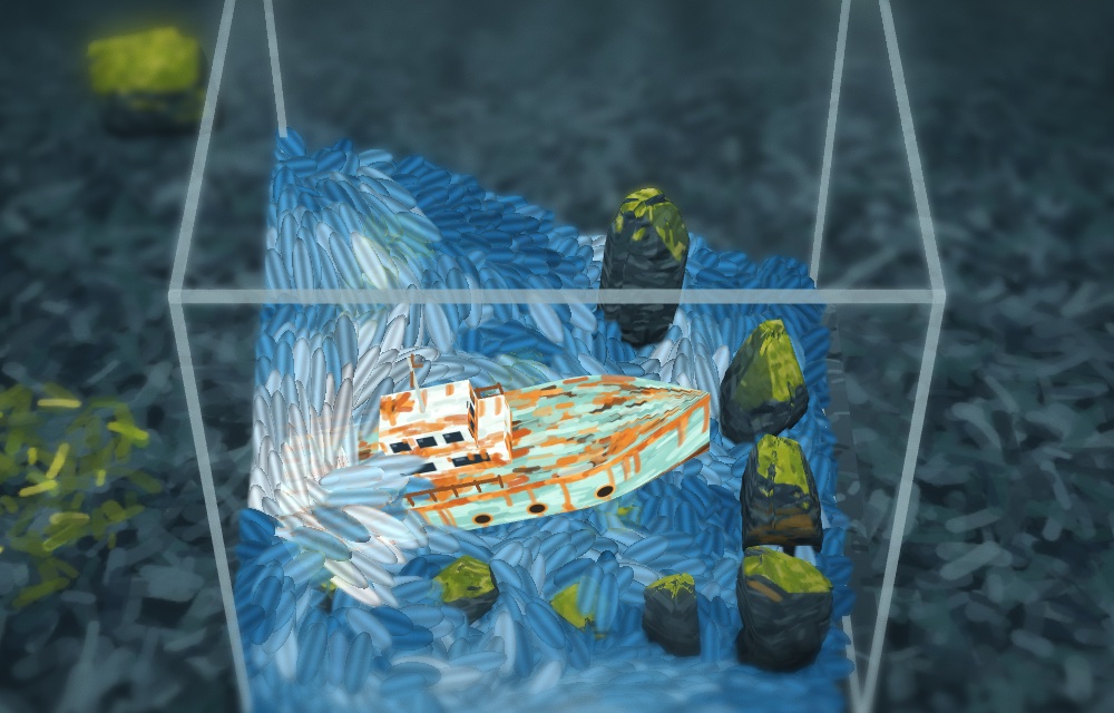
<p><img src="https://www.andrewklong.com/images/isle-of-savreen/wreck-and-boulders.jpg" alt="The rusting fishing boat lying bow-up in the tank among mossy slate boulders, with painted water piled up around its stern" /></p>

<p>The wreck comes from a painting of a beached fishing boat, pale teal paint
flaking to orange rust. It’s built in code: a hull lofted from cross-sections
narrowing to a raked bow, a deckhouse and wheelhouse, railings with posts
missing, and a leaning mast, painted with the same brush strokes as
everything else. The rocks are a reusable boulder model: give it a box and a
seed and it grows a unique rock in that box, with flat facets where slate has
split, layered ledges, clefts, a lean, and moss on whatever faces up.</p>

<p>The water meets them through <em>signed distance fields</em>: grids storing, at every
point, how far it is to the nearest surface, negative inside. Any shape that
can answer “is this point inside me?” can be baked into one, and step 3 above
becomes a single lookup per particle: if a drop is too close, push it out
along the direction the distance grows fastest. The mesh you see and the shape
the water hits come from the same function, so they always agree.</p>

<h2 id="from-physics-to-pixels">From physics to pixels</h2>

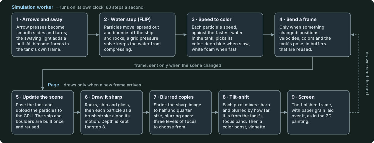
<p>The simulation and the drawing run on separate threads. A worker thread owns
the water and steps it 60 times a second on its own clock; the page only
draws, and only when the worker has sent something new:</p>

<p><img src="https://www.andrewklong.com/images/isle-of-savreen/rendering-pipeline.svg" alt="A diagram of the rendering pipeline in two lanes. The simulation worker, running 60 steps a second: 1, arrows and sway become forces in the tank's frame; 2, the water step moves the particles, keeps them apart and off the solids, and solves for pressure; 3, each particle's speed picks its color from deep blue to white foam; 4, a frame is sent only when something changed. An arrow carries the frame down to the page, which draws only when a new frame arrives: 5, update the scene and upload the particles; 6, draw the rocks, ship, glass and brush strokes sharp, keeping depth; 7, make half- and quarter-size blurred copies; 8, the tilt-shift pass mixes sharp and blurred by each pixel's distance from the focus band, then boosts color and adds a vignette; 9, show it on screen with paper grain. A dashed arrow returns from the screen to the worker: drawn, send the next." /></p>

<p>The model-railway look is a fake tilt-shift lens. A real one keeps only a
thin band of the scene sharp, which is what your eye expects of something a
few centimeters away. Here the scene is drawn sharp, blurred copies are made,
and each pixel picks its blur from how far it is from the tank, above, below,
in front or behind, with a little extra saturation and a vignette on top.</p>

<h2 id="quieting-the-fans">Quieting the fans</h2>

<p>The first version made my laptop sound like it was taking off, so I measured.
The surprise: two-thirds of each step went to step 2, pushing overlapping
particles apart, and only a few percent to the pressure solve. Sorting the
particles by grid cell, so neighbors sit next to each other in memory, and
checking each nearby pair once instead of twice made every step 35 to 40
percent faster.</p>

<p>The rest was wasted drawing. The screen runs at 120 frames a second, but the
water only changes 60 times a second, and the page kept redrawing even while
paused. Now the page draws only when the worker sends a new frame, and the
worker sleeps when nothing is moving. Idle, CPU use went from about three cores
to a third of one in a software-rendering test, and the water runs at real
speed whatever the frame rate.</p>

<h2 id="try-it">Try it</h2>

<p><a href="/IsleOfSavreen/">Isle of Savreen is live here</a>, and the code is on GitHub:
<a href="https://github.com/AndrewKL/IsleOfSavreen">AndrewKL/IsleOfSavreen</a>. It’s
TypeScript with three.js, a Web Worker for the simulation and the Web Audio
API for sound. Turn your sound on, click to start, then tip the tank: the
arrow keys slide it, Shift with the arrows tilts it, and Q and E spin it.</p>

<ul class="actions special">
  <li><a href="/IsleOfSavreen/" class="button large">Launch Isle of Savreen</a></li>
  <li><a href="https://github.com/AndrewKL/IsleOfSavreen" class="button large">View the code on GitHub</a></li>
</ul>]]></content><author><name></name></author><summary type="html"><![CDATA[The water simulator goes 3D: a glass cube of painted water with a rusting shipwreck and mossy boulders inside, seen like a tilt-shift photograph of a model. Tip, spin and slide the tank and the water answers. How FLIP turns a few thousand particles into water, how moving the tank becomes forces the water feels, and how I quieted my laptop's fans.]]></summary><media:thumbnail xmlns:media="http://search.yahoo.com/mrss/" url="https://www.andrewklong.com/images/isle-of-savreen/tank-diorama.jpg" /><media:content medium="image" url="https://www.andrewklong.com/images/isle-of-savreen/tank-diorama.jpg" xmlns:media="http://search.yahoo.com/mrss/" /></entry><entry><title type="html">Helios: the three-body problem in light and sound</title><link href="https://www.andrewklong.com/blog/helios-the-three-body-problem-in-light-and-sound/" rel="alternate" type="text/html" title="Helios: the three-body problem in light and sound" /><published>2026-09-25T00:00:00+00:00</published><updated>2026-09-25T00:00:00+00:00</updated><id>https://www.andrewklong.com/blog/helios-the-three-body-problem-in-light-and-sound</id><content type="html" xml:base="https://www.andrewklong.com/blog/helios-the-three-body-problem-in-light-and-sound/"><![CDATA[<ul class="actions special">
  <li><a href="/Helios3BodyProblemVisualizer/" class="button large">Launch Helios</a></li>
  <li><a href="https://github.com/AndrewKL/Helios3BodyProblemVisualizer" class="button large">View the code on GitHub</a></li>
</ul>

<p><a href="/Helios3BodyProblemVisualizer/">Helios</a> is a gravity sandbox that runs in the
browser. Click anywhere a few times to drop some bodies, press Play, and watch
them pull on each other. Every body is a glowing sphere that pulses and
hums a low sci-fi drone. The closer it gets to another body, the bigger and
brighter it gets and the faster it pulses and wubs. It never plays out the same way
twice, and that is the point: it is a toy built around one of the oldest
unsolved problems in physics.</p>

<h2 id="the-three-body-problem">The three-body problem</h2>

<p>Given three masses, their positions and their velocities, where will they be
at any later time? Newton answered this for <em>two</em> bodies in 1687. Two bodies
trace ellipses, parabolas or hyperbolas forever, and a formula tells you
exactly where they will be at any time you like. Add a third body and there is no such
formula.</p>

<h2 id="why-its-hard-to-solve">Why it’s hard to solve</h2>

<p>It is not for lack of trying. The problem has too many unknowns and too few
rules. Three bodies moving in space have 18 numbers that change over time:
three position and three velocity components each. Conservation of energy,
momentum and angular momentum pins down only 10 of them. In 1887 Heinrich
Bruns proved there are no other algebraic conserved quantities to make up the
difference.</p>

<p>Henri Poincaré went further around 1890 and showed that the motion generally
can’t be reduced to a neat formula at all. Karl Sundman did find an infinite
series that technically solves it, in 1912, but it converges so slowly that
it is useless in practice.</p>

<p>So we simulate. Astronomers step the bodies forward in small time increments,
computing the forces and nudging every position and velocity a little at a
time, and so does Helios. That works, but every step adds a tiny error, and
with three bodies tiny errors don’t stay tiny.</p>

<h2 id="why-its-unstable">Why it’s unstable</h2>

<p>Poincaré’s other discovery was chaos. A difference in starting positions far
smaller than you could ever measure grows exponentially over time. Two nearly
identical setups soon look nothing alike, so long-term prediction is
impossible even though the laws themselves are exact. Nothing is random here;
it is deterministic and still unpredictable.</p>

<p>The mechanism is the close encounter. When two bodies pass near each other
they swap a lot of energy very quickly, and one can be flung onto a wide
orbit or out of the system entirely. That is the usual ending: most
three-body systems eventually throw one body out, and the other two settle
into a tight pair carrying away the leftover energy.</p>

<p>There are rare exceptions, special starting positions that repeat forever.
Euler found three bodies in a line in 1767, and Lagrange found them at the
corners of an equilateral triangle in 1772; Jupiter’s Trojan asteroids ride
that triangle. In 1993 Cris Moore found three equal masses chasing each other
around a figure-eight. But most of these orbits are balanced on a knife-edge.
Nudge them and chaos takes over.</p>

<h2 id="science-art-and-music">Science, art and music</h2>

<p>Helios is honest physics. Every body pulls on every other body with Newton’s
inverse-square law, and a velocity Verlet integrator steps it forward 240
times a second, with a fixed timestep so the result doesn’t depend on your
frame rate. There are two deliberate compromises, and the info panel in the
app says so. Gravity is softened at very short range so bodies pass through
each other instead of reaching infinite speeds. And a weak attractor sits at
the center of the screen, pulling strays back instead of letting the usual
ejection end the show.</p>

<p>The art is in what the physics is made to look like. The quantity that
matters most in a three-body system is invisible: how close each body is to
its nearest neighbor, because that is where the close encounters, the energy
swaps and the chaos come from. Helios draws that. As two bodies approach,
each grows, its core burns whiter, its pulse speeds up and deepens, and it
stretches toward its neighbor like a body being pulled apart by tides. A near
miss reads as a flare. The drama on screen is the same thing that is making
the math hard.</p>

<p>The music does the same thing for your ears. Each body is its own voice: two
detuned sawtooth waves and a sub-octave sine running through a resonant
filter, with a slow oscillator sweeping the filter open and closed. That
sweep is the “wub.” Far from everything, a body wubs lazily, about one and a
half times a second. As it closes in on another body, the wub speeds up to
ten times a second and the tone gets brighter and louder. Each body is panned
left or right by its position on screen, so you can hear where it is.</p>

<p>The notes are chosen so the chaos stays listenable. Each new body takes the
next note of a pentatonic scale, the five-note scale with no half steps in
it, so however many bodies you add and however they move, the
chord never clashes. The physics decides the rhythm and the scale keeps the
harmony.</p>

<p>Put together, a simulation becomes a composition that no one wrote. You
choose the starting positions, and after that Newton writes the score: long
quiet drifts where every voice wubs slowly and apart, then a close pass where
two voices race and flare together, and one body gets slung across the stereo
field. Place the same bodies a few pixels differently and you get an entirely
different piece. That is chaos, heard rather than read about.</p>

<h2 id="try-it">Try it</h2>

<p><a href="/Helios3BodyProblemVisualizer/">Helios is live here</a>, and the code is on
GitHub:
<a href="https://github.com/AndrewKL/Helios3BodyProblemVisualizer">AndrewKL/Helios3BodyProblemVisualizer</a>.
It is TypeScript and three.js, with the Web Audio API for the sound and no
other libraries. Turn your sound on, click a handful of times, and press Play.</p>

<ul class="actions special">
  <li><a href="/Helios3BodyProblemVisualizer/" class="button large">Launch Helios</a></li>
  <li><a href="https://github.com/AndrewKL/Helios3BodyProblemVisualizer" class="button large">View the code on GitHub</a></li>
</ul>]]></content><author><name></name></author><summary type="html"><![CDATA[A gravity sandbox where every body glows, pulses and hums, and the closer two bodies get, the faster they pulse and wub. Why three bodies have no general solution, why they fly apart, and what happens when you turn a physics problem into something you can see and hear.]]></summary><media:thumbnail xmlns:media="http://search.yahoo.com/mrss/" url="https://www.andrewklong.com/images/helios/close-encounter.jpg" /><media:content medium="image" url="https://www.andrewklong.com/images/helios/close-encounter.jpg" xmlns:media="http://search.yahoo.com/mrss/" /></entry><entry><title type="html">Keeping big lists off the .NET heap</title><link href="https://www.andrewklong.com/blog/keeping-big-lists-off-the-dotnet-heap/" rel="alternate" type="text/html" title="Keeping big lists off the .NET heap" /><published>2026-09-25T00:00:00+00:00</published><updated>2026-09-25T00:00:00+00:00</updated><id>https://www.andrewklong.com/blog/keeping-big-lists-off-the-dotnet-heap</id><content type="html" xml:base="https://www.andrewklong.com/blog/keeping-big-lists-off-the-dotnet-heap/"><![CDATA[<ul class="actions special">
  <li><a href="https://github.com/AndrewKL/CSharpOffHeapStorage" class="button large">View the code on GitHub</a></li>
</ul>

<p>When I was a new SDE at ZS Associates, more than 15 years ago, I spent a
significant amount of time playing with very large in-memory lists. Calling
<code class="language-plaintext highlighter-rouge">ToList()</code> on a few million records is easy to write, and it’s easy to miss
what it costs: memory climbs, the garbage collector kicks in over and over,
and more and more of the program’s time goes to the runtime cleaning up
after it.</p>

<p>A few years later, in 2014, I wrote a small library to test an idea: what if
the list didn’t live on the managed heap at all? Serialize every object into
one big block of memory, and turn the bytes back into objects only while you
are looping over them. I recently got it building again on .NET 10, moved its
storage into native memory, and wrote a benchmark to see whether the idea
holds up.</p>

<h2 id="why-a-big-list-hurts">Why a big list hurts</h2>

<p>.NET’s garbage collector is generational. New objects start in generation 0,
which is collected often and cheaply, on the bet that most objects die young.
Objects that survive a few collections get promoted to generation 2, which is
only collected occasionally. To collect, the GC has to find every object that
is still reachable, which means following every reference from every live
object. The cost of that tracing grows with the number of live objects, not
with how much memory they take up.</p>

<p>A big list breaks the generational bet. Every record you add survives, because
the list holds on to it. So each gen 0 collection finds almost nothing to free
and has to copy the survivors up a generation, and the gen 1 and gen 2
collections that follow have to trace millions of objects and references each
time. Five million records with one string each is ten million objects, plus
the list’s internal array, which is big enough to go on the Large Object Heap.
Every one of those objects also carries a 16-byte header and is reached
through an 8-byte pointer.</p>

<p>None of this shows up as an error. The program just gets slower, and it gets
slower the most in the code that has nothing to do with the list, because a
long gen 2 collection pauses every thread.</p>

<h2 id="getting-the-data-off-the-heap">Getting the data off the heap</h2>

<p>The library is <code class="language-plaintext highlighter-rouge">OffHeapIEnumerable&lt;T&gt;</code>. You give it any <code class="language-plaintext highlighter-rouge">IEnumerable&lt;T&gt;</code>, and
it walks through it once, writing each object’s properties into a stream with
a <code class="language-plaintext highlighter-rouge">BinaryWriter</code>: an <code class="language-plaintext highlighter-rouge">int</code> is 4 bytes, a <code class="language-plaintext highlighter-rouge">string</code> is a length prefix plus
UTF-8, and so on. Enumerating it reads the stream back and builds a fresh
object for each record as you reach it. To the GC, the whole data set is
nothing but the stream.</p>

<p>What that stream sits on has changed three times. The first version used a
plain <code class="language-plaintext highlighter-rouge">MemoryStream</code>, which keeps everything in one <code class="language-plaintext highlighter-rouge">byte[]</code>. That fails on
big data sets, because a single array needs one contiguous run of memory and
a <code class="language-plaintext highlighter-rouge">MemoryStream</code> can’t grow past 2 GB. The 2014 version swapped in a
<code class="language-plaintext highlighter-rouge">MemoryTributary</code>, which is a stream backed by a list of 64 KB arrays. The
chunks are small enough to stay off the Large Object Heap, and the GC only
sees a few thousand of them instead of millions of objects. They are still
managed memory, though.</p>

<p>The version I have now allocates its 1 MB blocks with <code class="language-plaintext highlighter-rouge">NativeMemory.Alloc</code>,
outside the GC heap entirely. The GC never scans them, never moves them and
doesn’t count them. The catch is that nothing frees them for you. The
collection is <code class="language-plaintext highlighter-rouge">IDisposable</code>, and you have to dispose it, the same as a file
handle.</p>

<h2 id="the-benchmark">The benchmark</h2>

<p>The benchmark builds 5 million records, each with an <code class="language-plaintext highlighter-rouge">int</code>, a <code class="language-plaintext highlighter-rouge">string</code>, a
<code class="language-plaintext highlighter-rouge">decimal</code>, a <code class="language-plaintext highlighter-rouge">double</code> and a <code class="language-plaintext highlighter-rouge">bool</code>, and stores them three ways. The first is a
plain <code class="language-plaintext highlighter-rouge">List&lt;T&gt;</code>. The second is the off-heap collection with the original
serializer. The third is the off-heap collection with a newer, faster
serializer I’ll come back to. For each one it measures how long it takes to
build, how long it takes to loop over once, how much memory it holds, and how
long a forced full, blocking garbage collection takes while the data is still
alive. That last number is the one this whole project is about.</p>

<table>
  <thead>
    <tr>
      <th> </th>
      <th style="text-align: right"><code class="language-plaintext highlighter-rouge">List&lt;T&gt;</code></th>
      <th style="text-align: right">Off heap, boxed</th>
      <th style="text-align: right">Off heap, typed</th>
    </tr>
  </thead>
  <tbody>
    <tr>
      <td>Build</td>
      <td style="text-align: right">1,503 ms</td>
      <td style="text-align: right">546 ms</td>
      <td style="text-align: right">476 ms</td>
    </tr>
    <tr>
      <td>Time in GC pauses while building</td>
      <td style="text-align: right">916 ms</td>
      <td style="text-align: right">29 ms</td>
      <td style="text-align: right">23 ms</td>
    </tr>
    <tr>
      <td>Gen 2 collections while building</td>
      <td style="text-align: right">6</td>
      <td style="text-align: right">0</td>
      <td style="text-align: right">0</td>
    </tr>
    <tr>
      <td>Memory held</td>
      <td style="text-align: right">560 MB</td>
      <td style="text-align: right">204 MB</td>
      <td style="text-align: right">204 MB</td>
    </tr>
    <tr>
      <td>Full GC while the data is alive</td>
      <td style="text-align: right">124 ms</td>
      <td style="text-align: right">0.1 ms</td>
      <td style="text-align: right">0.2 ms</td>
    </tr>
    <tr>
      <td>Enumerate once</td>
      <td style="text-align: right">84 ms</td>
      <td style="text-align: right">749 ms</td>
      <td style="text-align: right">392 ms</td>
    </tr>
  </tbody>
</table>

<p>The off-heap version is three times faster to build, and the reason is in the
second row. More than half of the <code class="language-plaintext highlighter-rouge">List&lt;T&gt;</code> build time is the garbage
collector copying and tracing records that were never going to die. The
off-heap version makes plenty of garbage while building too, but all of it
dies young, which is the case the GC is designed for.</p>

<p>It also takes 2.7 times less memory. The list pays a 16-byte header for every
record and every string, an 8-byte pointer to each, and two bytes per character
in UTF-16. The stream pays a byte or two of framing instead.</p>

<p>A full collection with the list alive takes 124 ms, and that grows with the
list. With the data off heap it takes a tenth of a millisecond, because
there’s nothing left to trace.</p>

<p>And then there’s the last row. Looping over the list takes 84 ms, because the
objects are already there. Looping over the off-heap version is about 5 to 9
times slower, because every pass has to build 5 million new objects and 5 million
new strings from bytes.</p>

<h2 id="boxing-and-a-faster-serializer">Boxing, and a faster serializer</h2>

<p>The original serializer made that last row worse than it needed to be. It
worked through reflection in the most general way: a list of properties, each
with a getter and setter delegate typed as <code class="language-plaintext highlighter-rouge">object</code>, and a <code class="language-plaintext highlighter-rouge">switch</code> on the
property’s type. Every <code class="language-plaintext highlighter-rouge">int</code>, <code class="language-plaintext highlighter-rouge">bool</code>, <code class="language-plaintext highlighter-rouge">decimal</code> and <code class="language-plaintext highlighter-rouge">double</code> it read got boxed
into a short-lived heap object on the way to its setter. That’s four extra
allocations and five delegate calls per record.</p>

<p>The typed serializer builds one reader and one writer per type with
expression trees and compiles them, so the result is the same code you would
write by hand:</p>

<div class="language-csharp highlighter-rouge"><div class="highlight"><pre class="highlight"><code><span class="n">reader</span> <span class="p">=&gt;</span> <span class="k">new</span> <span class="n">Record</span>
<span class="p">{</span>
    <span class="n">Id</span> <span class="p">=</span> <span class="n">reader</span><span class="p">.</span><span class="nf">ReadInt32</span><span class="p">(),</span>
    <span class="n">Name</span> <span class="p">=</span> <span class="n">reader</span><span class="p">.</span><span class="nf">ReadBoolean</span><span class="p">()</span> <span class="p">?</span> <span class="n">reader</span><span class="p">.</span><span class="nf">ReadString</span><span class="p">()</span> <span class="p">:</span> <span class="k">null</span><span class="p">,</span>
    <span class="n">Price</span> <span class="p">=</span> <span class="n">reader</span><span class="p">.</span><span class="nf">ReadDecimal</span><span class="p">(),</span>
    <span class="n">Score</span> <span class="p">=</span> <span class="n">reader</span><span class="p">.</span><span class="nf">ReadDouble</span><span class="p">(),</span>
    <span class="n">Active</span> <span class="p">=</span> <span class="n">reader</span><span class="p">.</span><span class="nf">ReadBoolean</span><span class="p">()</span>
<span class="p">}</span>
</code></pre></div></div>

<p>That halves the garbage made while enumerating, down to exactly one record
and one string each, and it makes enumeration 1.3 to 1.9 times faster across
runs. It is still slower than walking a list. Most of the remaining cost is
going through <code class="language-plaintext highlighter-rouge">BinaryReader</code> and <code class="language-plaintext highlighter-rouge">Stream</code> for every 4- or 8-byte field; reading
straight out of the native blocks would be the next step.</p>

<h2 id="on-heap-vs-off-heap">On heap vs off heap</h2>

<p><strong>On heap</strong> is the right default, and it isn’t close for most programs.</p>

<ul>
  <li>Reading is as fast as it gets. The objects already exist, so a loop is just
following pointers.</li>
  <li>You get random access, updates in place, LINQ, and any type you like,
including ones with nested objects and collections.</li>
  <li>The GC frees it all for you, and there is no serialization format to keep in
sync with your classes.</li>
  <li>The cost is the GC. Every live object is something to trace, so collections
get slower as the data grows, and it’s the whole process that pauses, not
just the code using the list.</li>
  <li>Small objects are memory-hungry: 16 bytes of header each, 8 bytes per
reference, and UTF-16 strings.</li>
</ul>

<p><strong>Off heap</strong> trades read speed for everything else.</p>

<ul>
  <li>A full GC stays at a tenth of a millisecond no matter how much data you
hold, and building the data set doesn’t push the rest of the program through
gen 2 collections.</li>
  <li>It takes much less memory, because there are no object headers or
pointers, and strings are stored as UTF-8.</li>
  <li>Every read deserializes. If you loop over the data many times, you pay that
cost every time, and it is several times the cost of reading a list.</li>
  <li>It only goes forward. There’s no indexing and no updating in place; you
append and you enumerate.</li>
  <li>It only handles the types the serializer knows about. Here that’s <code class="language-plaintext highlighter-rouge">int</code>,
<code class="language-plaintext highlighter-rouge">bool</code>, <code class="language-plaintext highlighter-rouge">decimal</code>, <code class="language-plaintext highlighter-rouge">float</code>, <code class="language-plaintext highlighter-rouge">double</code> and <code class="language-plaintext highlighter-rouge">string</code> properties on a class with
a public parameterless constructor.</li>
  <li>You own the memory. Forget to dispose it and the GC won’t know it’s there,
so the finalizer that would eventually free it may not run for a long time.</li>
  <li>The objects you get back are copies. Changing one doesn’t change what’s
stored.</li>
</ul>

<p>The trade is worth it when the data set is big, lives a long time, is read
only a few times, and shares a process with code that cares about pause
times, like a web server that keeps a large cache or reference data set in
memory. It isn’t worth it for a list you build, loop over once and throw away.
A few million short-lived objects are exactly what the GC is good at.</p>

<h2 id="what-id-reach-for-today">What I’d reach for today</h2>

<p>There are other ways to get most of the way there. Background GC does most
of the gen 2 work while your threads keep running, although the gen 0 and
gen 1 collections that promote a growing list still stop them. If your records can be <code class="language-plaintext highlighter-rouge">struct</code>s with no reference fields, an array of
them is one object to the GC, and the GC doesn’t look inside it, which gets
you most of the benefit with none of the serialization. And if the data is
really a table, an in-process columnar engine like DuckDB, or Apache Arrow,
will do this better than a hand-rolled stream.</p>

<p>Still, the core idea holds. The garbage collector’s cost is in the number of
live objects, not their size, so when you have millions of them, the best
thing you can do is give it fewer to look at.</p>

<p>The code, the tests and the benchmark are on GitHub at
<a href="https://github.com/AndrewKL/CSharpOffHeapStorage">AndrewKL/CSharpOffHeapStorage</a>.
Running
<code class="language-plaintext highlighter-rouge">dotnet run -c Release --project OffHeapStorage.Benchmark -- 1000000 5000000</code>
reproduces the numbers on your own machine.</p>

<ul class="actions special">
  <li><a href="https://github.com/AndrewKL/CSharpOffHeapStorage" class="button large">View the code on GitHub</a></li>
</ul>]]></content><author><name></name></author><summary type="html"><![CDATA[Millions of small objects in a List are cheap to read and expensive to keep around, because the garbage collector has to trace every one of them. Serializing them into native memory instead cuts memory use by almost two-thirds and makes a full GC almost free, but every read gets slower. A small C# library, a benchmark and the trade-offs.]]></summary><media:thumbnail xmlns:media="http://search.yahoo.com/mrss/" url="https://www.andrewklong.com/images/off-heap/benchmark.jpg" /><media:content medium="image" url="https://www.andrewklong.com/images/off-heap/benchmark.jpg" xmlns:media="http://search.yahoo.com/mrss/" /></entry><entry><title type="html">Painting water with the Navier–Stokes equations</title><link href="https://www.andrewklong.com/blog/painting-water-with-the-navier-stokes-equations/" rel="alternate" type="text/html" title="Painting water with the Navier–Stokes equations" /><published>2026-09-25T00:00:00+00:00</published><updated>2026-09-25T00:00:00+00:00</updated><id>https://www.andrewklong.com/blog/painting-water-with-the-navier-stokes-equations</id><content type="html" xml:base="https://www.andrewklong.com/blog/painting-water-with-the-navier-stokes-equations/"><![CDATA[<ul class="actions special">
  <li><a href="/NavierStokesSimulation/" class="button large">Launch the water simulator</a></li>
  <li><a href="https://github.com/AndrewKL/NavierStokesSimulation" class="button large">View the code on GitHub</a></li>
</ul>

<p>The <a href="/NavierStokesSimulation/">water simulator</a> is a small river that runs in
the browser. Click once and water pours from a ledge high on the left, crashes
onto a row of mossy boulders, pools behind them, spills over and runs out the
right side. Drag anywhere to drop in a new boulder and watch the water find
its way around it. The whole scene is painted in brush strokes: still water is
deep blue, and the faster the water moves, the paler it gets, until the
fastest water on screen is white foam. It sounds like water too, with a rush
that follows the current, splashes where it lands, and a low surf that swells
as it sloshes.</p>

<h2 id="the-navierstokes-equations">The Navier–Stokes equations</h2>

<p>Water, air, honey and blood all move by the same two rules. Claude-Louis Navier
wrote them down in 1822 and George Gabriel Stokes put them on firm footing in</p>
<ol>
  <li>They are Newton’s <em>force equals mass times acceleration</em>, applied to
every tiny parcel of a fluid.</li>
</ol>

<p>The first rule is about momentum. A parcel of water speeds up or turns because
pressure pushes on it, gravity pulls on it, and viscosity, the fluid’s internal
friction, drags it toward the speed of its neighbors. It also carries its own
velocity along as it moves, and that self-carrying term is what makes flow
curl back on itself into swirls and eddies.</p>

<p>The second rule is that water can’t be squeezed. Whatever flows into any small
region has to flow out again. Pressure is exactly the force needed to keep
that true: it builds up wherever water is being crammed together and pushes
it apart.</p>

<h2 id="why-theyre-still-unsolved">Why they’re still unsolved</h2>

<p>Two short equations, and still nobody knows whether they always make sense. In
three dimensions, no one has proved that smooth solutions always exist, or
that the velocity can’t suddenly blow up to infinity at a point. It is one of
the Clay Mathematics Institute’s seven Millennium Prize Problems, with a
million-dollar reward for either answer.</p>

<p>The practical problem is turbulence. How chaotic a flow gets depends on its
Reynolds number: speed times size, divided by viscosity. A stream running at a
meter per second over a meter-sized rock has a Reynolds number around a
million. At that point the flow breaks into eddies, the eddies break into
smaller eddies, and the cascade doesn’t stop until it reaches swirls tens of
microns across, where viscosity finally turns the motion into heat. Resolving
all of that in 3D would take something like ten trillion grid cells. Engineers
don’t do it. They model the small eddies statistically and simulate only the
big ones, and even that takes supercomputers.</p>

<h2 id="how-a-few-thousand-particles-fake-a-waterfall">How a few thousand particles fake a waterfall</h2>

<p>This simulation cheats in the way film effects cheat. It uses a method called
FLIP, short for Fluid-Implicit-Particle. Brackbill and Ruppel invented it for
plasma physics in 1986, and Zhu and Bridson brought it to computer graphics in</p>
<ol>
  <li>The water is about six thousand particles, each carrying a position and
a velocity. Every step, their velocities are copied onto a coarse 120 × 60
grid. A pressure solve adjusts the grid until no cell gains or loses water,
and the change is copied back to the particles. The particles give you a free
surface, where water meets air, for free, and they carry momentum without
smearing it, which is what keeps the water lively and splashy instead of
syrupy.</li>
</ol>

<p>It looks right because at this scale water is dominated by gravity, inertia
and incompressibility, and FLIP gets those three right. Jets fall in
parabolas, pools find their level, waves travel and water piles up against
rocks. What it gets wrong is everything small. There is no viscosity term, the
only damping comes from numerical side effects, and the grid cells are about a
thousand times too coarse to see real turbulence. It is also 2D, and 2D
turbulence is a different animal: small swirls merge into big, long-lived
whirlpools instead of shattering into smaller ones. The big lazy eddies you
see in the pools are partly that.</p>

<h2 id="science-art-and-sound">Science, art and sound</h2>

<p>The physics decides where every bit of water goes. The art is in what it is
made to look like, and the look comes from an impasto painting of a woodland
waterfall: white water tumbling between dark slate boulders with bright moss
on top.</p>

<p>Color is speed. The quantity your eye can’t normally see in moving water is
how fast each part of it is going, so the simulation paints it. Each particle’s
speed is compared with the fastest water currently in the scene. The slowest
water is deep blue, faster water is paler, and the fastest is white. The scale
follows the water, so a gentle trickle and a torrent both use the full range.
Press Surge and the whole jet flashes white, then the colors settle back over
a second or two as the scale catches up. This happens to be how rivers look.
Real white water is white because it is fast and broken up, and still pools
are dark.</p>

<p>Every particle is a brush stroke. Each one is stretched along the direction
it is moving, with bristle streaks and a little variation in tone, so fast
water becomes long, thin, pale streaks that trace the flow, and still water
becomes short horizontal dabs, like a painter’s pool. The rocks are painted
the same way: slate strokes with light catching the top, a band of moss that
creeps down the sides, and a seed per rock so it looks the same every frame.</p>

<p>The sound is built the same way, from the physics up, with no recorded audio
at all. A rush of filtered noise follows the average speed of the water,
getting louder and brighter as it speeds up, and pans toward wherever the fast
water is. Splashes are short bursts of noise, triggered when water hits
something hard enough to change its velocity sharply. Under both is a low surf
that swells and fades like waves on a shore and grows as the water sloshes up
and down. Draw a boulder into a quiet pool and you hear the slap. Press Surge
and the whole river roars.</p>

<h2 id="try-it">Try it</h2>

<p><a href="/NavierStokesSimulation/">The water simulator is live here</a>, and the code is
on GitHub:
<a href="https://github.com/AndrewKL/NavierStokesSimulation">AndrewKL/NavierStokesSimulation</a>.
It is TypeScript and WebGL2, with the Web Audio API for the sound and no other
libraries. Turn your sound on, click to let the water flow, and drag a few
boulders into its path.</p>

<ul class="actions special">
  <li><a href="/NavierStokesSimulation/" class="button large">Launch the water simulator</a></li>
  <li><a href="https://github.com/AndrewKL/NavierStokesSimulation" class="button large">View the code on GitHub</a></li>
</ul>]]></content><author><name></name></author><summary type="html"><![CDATA[A 2D water simulation that pours over mossy rocks, painted in brush strokes that run from deep blue to white foam the faster the water moves, with a rush, splashes and a swelling surf you can hear. What the Navier–Stokes equations say, why they are still unsolved, and how a few thousand particles fake a waterfall.]]></summary><media:thumbnail xmlns:media="http://search.yahoo.com/mrss/" url="https://www.andrewklong.com/images/navier-stokes/painted-waterfall.jpg" /><media:content medium="image" url="https://www.andrewklong.com/images/navier-stokes/painted-waterfall.jpg" xmlns:media="http://search.yahoo.com/mrss/" /></entry><entry><title type="html">A data mesh for Amazon’s finance data</title><link href="https://www.andrewklong.com/blog/data-mesh-at-amazon-finance-automation/" rel="alternate" type="text/html" title="A data mesh for Amazon’s finance data" /><published>2026-09-24T00:00:00+00:00</published><updated>2026-09-24T00:00:00+00:00</updated><id>https://www.andrewklong.com/blog/data-mesh-at-amazon-finance-automation</id><content type="html" xml:base="https://www.andrewklong.com/blog/data-mesh-at-amazon-finance-automation/"><![CDATA[<p>I co-wrote a post on the AWS Big Data Blog with Nitin Arora, Kumar Satyen
Gaurav, Pradeep Misra and Rajesh Rao:
<a href="https://aws.amazon.com/blogs/big-data/how-amazon-finance-automation-built-a-data-mesh-to-support-distributed-data-ownership-and-centralize-governance/">How Amazon Finance Automation built a data mesh to support distributed data
ownership and centralize governance</a>.
I was the lead developer on it.</p>

<p>The problem is one every large finance organization eventually runs into.
Financial transactions used to fit on a single relational database. They
stopped fitting a long time ago, and the data ended up spread across a lot of
teams — each of which understood its own data best, and none of which wanted
to wait on a central team to publish it.</p>

<p>A data mesh is the usual answer: let the teams that own the data own the
publishing too, and centralize the governance rather than the data. The
interesting part is what that costs. Democratizing data product creation
removes the central bottleneck, but it hands every producer a new job —
onboarding a dataset to the catalog, then managing permissions on it, before
anyone else can use it. Get that wrong and adoption quietly stalls, because
the path of least resistance goes back to copying data around.</p>

<p>So most of the work went into making the obligations cheap. Producer accounts
sync their AWS Glue Data Catalog metadata into a central catalog. Lake
Formation in a central governance account holds the fine-grained permissions.
Consumers browse a front-end application, request access, and the request
routes to the data owner for approval, with a ticket behind it for auditing.
On approval, automation provisions an AWS RAM resource share, and the consumer
queries the data with Redshift Spectrum, Athena, EMR or QuickSight.</p>

<p>It currently hosts around 850 discoverable datasets and more than 300 curated
data products.</p>

<p>The diagram above is the shape of it: metadata copies inward in blue,
permissions flow outward in red, and no bulk data moves between the accounts
at all. The post has the rest of the diagrams and the details on the catalog
sync, which is the part that took the most care.</p>]]></content><author><name></name></author><summary type="html"><![CDATA[I co-wrote a post on the AWS Big Data Blog about the data mesh we built at Amazon Finance Automation, where I was the lead developer.]]></summary><media:thumbnail xmlns:media="http://search.yahoo.com/mrss/" url="https://www.andrewklong.com/images/data-mesh/architecture.jpg" /><media:content medium="image" url="https://www.andrewklong.com/images/data-mesh/architecture.jpg" xmlns:media="http://search.yahoo.com/mrss/" /></entry><entry><title type="html">Radmap: visualizing molecular reactivity with isodistance potential energy surfaces</title><link href="https://www.andrewklong.com/blog/radmap/" rel="alternate" type="text/html" title="Radmap: visualizing molecular reactivity with isodistance potential energy surfaces" /><published>2017-10-31T00:00:00+00:00</published><updated>2017-10-31T00:00:00+00:00</updated><id>https://www.andrewklong.com/blog/radmap</id><content type="html" xml:base="https://www.andrewklong.com/blog/radmap/"><![CDATA[<ul class="actions special">
  <li><a href="https://doi.org/10.1016/j.jmgm.2016.01.002" class="button large">Read the paper</a></li>
  <li><a href="https://github.com/AndrewKL/RADMAP" class="button large">View the code on GitHub</a></li>
</ul>

<p>When a free radical meets a molecule, where does it attack? For benzene the
answer is obvious, because every carbon is the same. For azulene, pyrene or a
new ligand nobody has made before, it isn’t, and finding out in the lab
takes time, material and sometimes a particle accelerator.</p>

<p>Radmap is a program I wrote as a chemistry student at Saint Mary’s
University in Halifax, in the Atlantic Centre for Green Chemistry, to answer
that question computationally. It shows the earliest moment of a reaction
between a molecule and a single atom (a hydrogen atom, a proton, a hydride, a
bromine atom or anything else monoatomic) as a colored surface wrapped
around the molecule. Red marks the low-energy spots, where the incoming atom
is drawn in and a radical is most likely to add.</p>

<p>We described the method in the <em>Journal of Molecular Graphics and
Modelling</em>:</p>

<blockquote>
  <p>Andrew K. Long, Jason A. Fawcett, Jason A.C. Clyburne and Cory C. Pye.
<a href="https://doi.org/10.1016/j.jmgm.2016.01.002">RADMAP: Simple probes for rapid assessment of complex reactivity: A method
and case studies on the reaction of hydrogen atoms with unsaturated organic
molecules</a>. <em>J. Mol. Graph.
Model.</em> <strong>64</strong>, 147–152 (2016).</p>
</blockquote>

<h2 id="why-muons">Why muons</h2>

<p>The problem came from muon chemistry. A positive muon that captures an
electron forms muonium, which behaves chemically like a hydrogen atom with
about a ninth of the mass. Fire muons into a sample and the muonium adds to
the molecules in it, just as a hydrogen atom would. In a transverse-field muon
spin resonance (µSR) experiment, each distinct radical that forms gives its
own pair of signals.</p>

<p>So before running an experiment you want to know how many places the muonium
can add, and roughly how much of each adduct will form. That tells you how
many signals to look for and how strong each should be. Beam time at a muon
facility is scarce, and a good prediction makes it go further.</p>

<h2 id="how-it-works">How it works</h2>

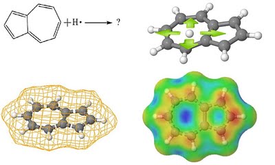
<p><img src="https://www.andrewklong.com/images/radmap/radmap-scan.jpg" alt="Four panels explaining Radmap. Top left: the question, azulene plus a hydrogen atom gives what? Top right: a 3D model of azulene with a hydrogen atom placed above it and arrows showing the atom being moved around the molecule. Bottom left: azulene inside an orange wireframe surface. Bottom right: the same surface filled in and colored from blue to red." />
<em>Azulene + H·: the question, a probe atom moved over the molecule, the
surface it samples, and the finished map.</em></p>
<p>Radmap works in four steps:</p>

<ol>
  <li><strong>Build a surface.</strong> Starting from a structure loaded from a <code class="language-plaintext highlighter-rouge">.mol</code> file,
Radmap draws a solvent-accessible surface around the molecule. Every point
on it sits a fixed distance outside the atoms (by default a 1.2 Å probe
radius beyond each atom’s van der Waals radius), which is what
<em>isodistance</em> means here. A resolution setting controls how many points
the mesh has.</li>
  <li><strong>Place the probe.</strong> For every point on the mesh, Radmap writes a Gaussian
input file containing the molecule plus the probe atom at that point, and
a batch file to run them all. You choose the probe, the charge and
multiplicity, and the method and basis set. The default is a short
two-step optimization at the unrestricted B3LYP/6-31G level, which suits
an open-shell radical.</li>
  <li><strong>Compute.</strong> Gaussian runs every job. This is the slow part: one quantum
chemistry calculation per point on the surface, which is why the batch
file can be split across machines.</li>
  <li><strong>Paint.</strong> Radmap reads the energy out of each output file, smooths the
values onto the displayed surface with a Gaussian-weighted average, and
colors it from blue (high energy, where the probe is pushed away) to red
(low energy, where the probe is drawn in).</li>
</ol>

<p>The result is a potential energy surface that isn’t a flat slice through
space but wraps the whole molecule, so every side of it can be compared
at once. The red regions predict where addition happens. The relative
energies of the red spots also give a qualitative estimate of how much of
each adduct forms, which says something about the molecule’s kinetic
stability as well as its reactivity.</p>

<p>The interface is built on <a href="https://jmol.sourceforge.net/">Jmol</a>, the open
source molecular viewer, so the finished map can be rotated and inspected
like any other Jmol model. Radmap itself is open source too.</p>

<h2 id="reading-the-maps">Reading the maps</h2>

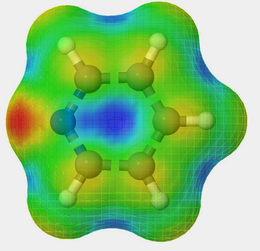
<p><img src="https://www.andrewklong.com/images/radmap/radmap-pyridine-hydrogen-radical.jpg" alt="Radmap surface around pyridine, mostly green and blue, with a strong red patch just outside the nitrogen atom and blue over the center of the ring." />
<em>Pyridine + H·. The strongest red sits just outside the nitrogen, and the
center of the ring is blue.</em></p>
<p>Pyridine is a good first example because it has only one feature that
isn’t a C–H. The map picks it out straight away: the hot spot is at the
nitrogen, and the ring carbons are all much cooler.</p>

<p><img src="https://www.andrewklong.com/images/radmap/radmap-pyrene-hdot-white.jpg" alt="Radmap surface around pyrene, with red patches over the outer carbon atoms, strongest on the upper and lower double bonds and at the carbons nearest the ring junctions, and blue over the center of each ring." />
<em>Pyrene + H·. Red over the outer carbons, weaker at the 2 and 7 positions,
and blue over the ring centers.</em></p>
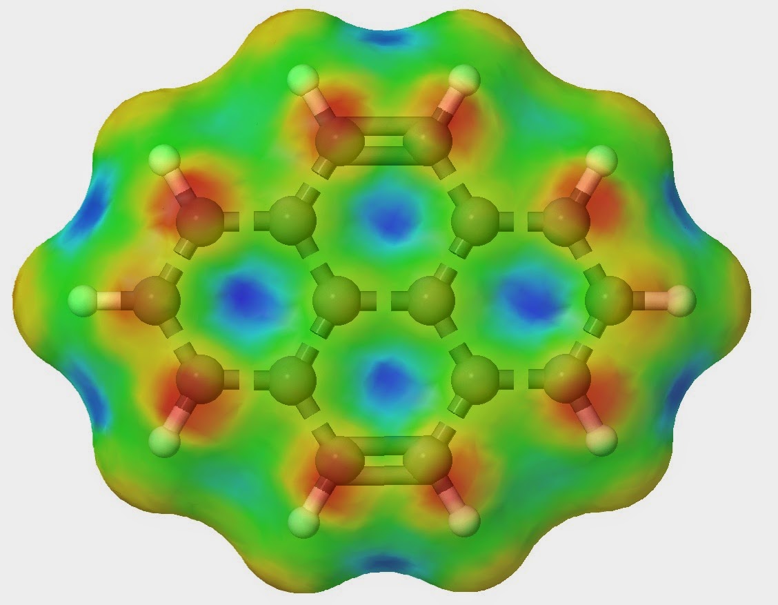
<p>Pyrene is where the method starts to earn its keep. It has 10 C–H carbons,
and the map separates them into groups: the carbons at the ends of the
upper and lower double bonds and the carbons next to the ring junctions
glow red, while the carbons in the middle of the left and right edges are
noticeably cooler. Each distinct red site is a distinct radical, and a
distinct µSR signal.</p>

<p><img src="https://www.andrewklong.com/images/radmap/radmap-cs2-opt.jpg" alt="Radmap surface around carbon disulfide, a linear S=C=S molecule. The surface is red at both sulfur ends, has blue bands over the carbon–sulfur bonds, and is green in the middle over the carbon." />
<em>Carbon disulfide + H·. The low-energy regions are the caps over the two
sulfur atoms, not the carbon.</em></p>
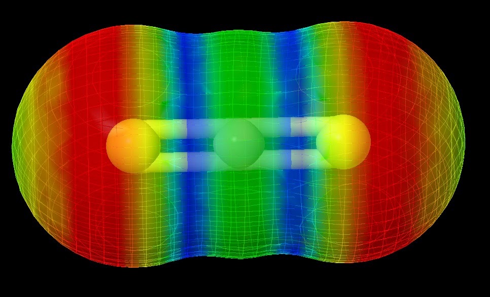
<p><img src="https://www.andrewklong.com/images/radmap/radmap-dimethylimidazole.jpg" alt="Radmap surface around 1,3-dimethylimidazol-2-ylidene, a five-membered ring with two N-methyl groups. A red patch sits over the carbene carbon between the two nitrogens, and the rest of the surface is green and blue." />
<em>1,3-Dimethylimidazol-2-ylidene, an N-heterocyclic carbene, + H·. The red
patch is over the carbene carbon between the two nitrogens.</em></p>
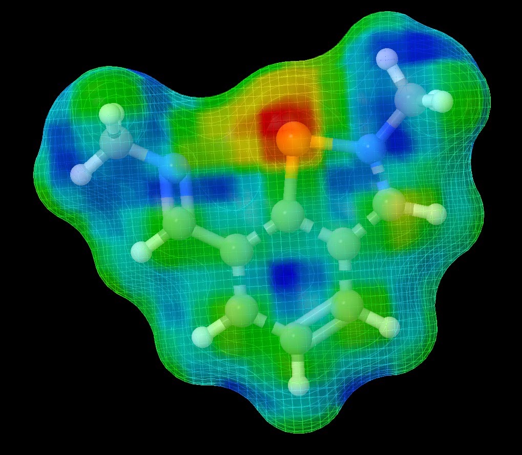
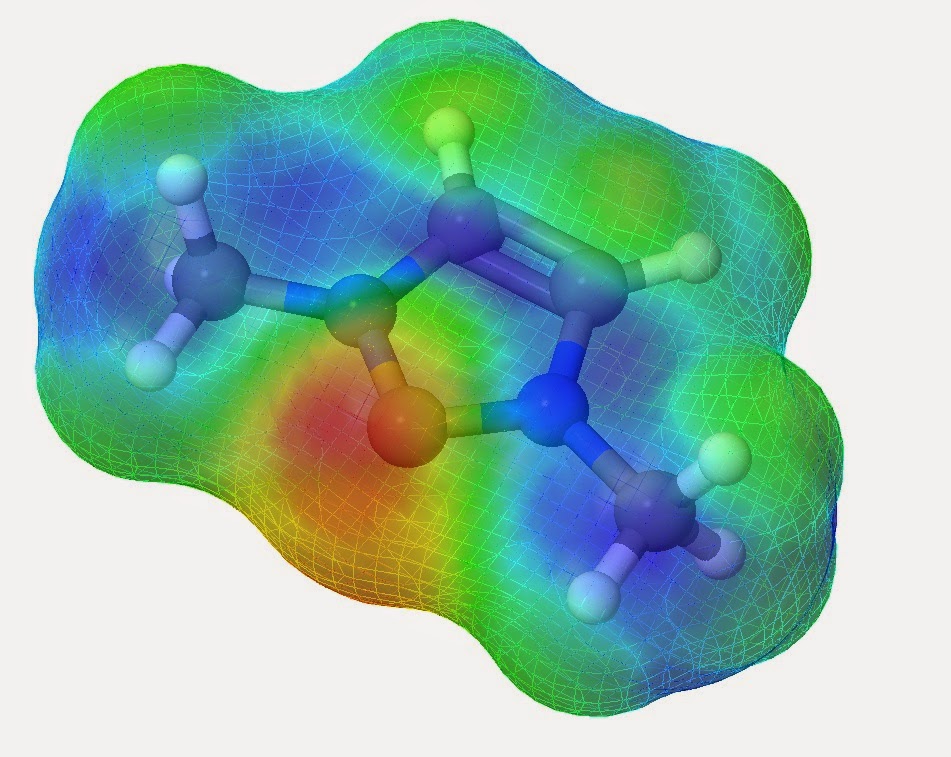
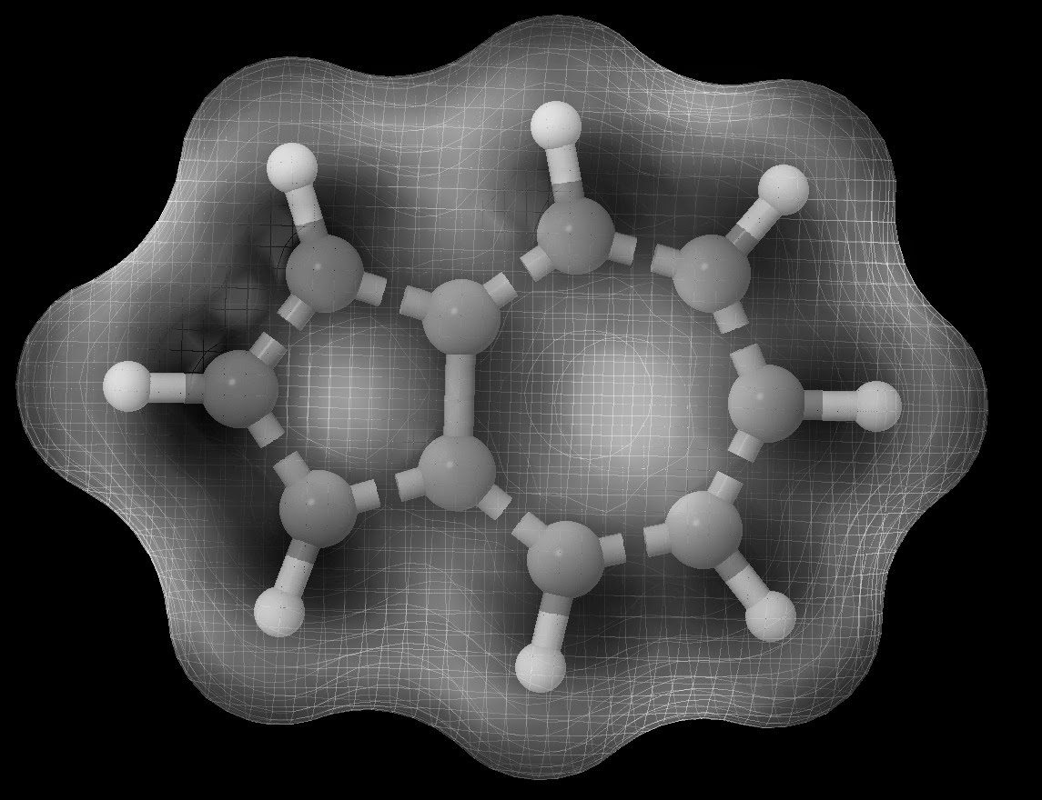
<p>The carbene is a nice check. Earlier muonium experiments from the Clyburne
group, with Paul Percival’s team, <a href="https://doi.org/10.1021/ja028770t">showed that the hydrogen atom adds to the
carbene carbon</a>, and that is exactly where
Radmap puts the red.</p>

<p><img src="https://www.andrewklong.com/images/radmap/radmap-p-pincer-low-rez.jpg" alt="Radmap surface around a phosphorus pincer compound. A single strong red patch sits over the central phosphorus atom, and the rest of the surface is green and blue." />
<em>A phosphorus pincer compound + H·. The reactive site is the phosphorus at
the center.</em></p>
<p>This is also where Radmap is useful beyond muons. When you design a new
ligand to bind to a metal, you want to know where its reactive sites are
before you spend weeks making it. A Radmap surface, run with whichever probe
fits the question, gives a quick first look.</p>

<p><img src="https://www.andrewklong.com/images/radmap/radmap-azulene-BW.jpg" alt="Radmap surface around azulene, rendered in grayscale, showing the smooth mesh that wraps the five- and seven-membered rings." />
<em>Azulene, rendered in grayscale.</em></p>

<h2 id="limitations">Limitations</h2>

<p>Radmap is deliberately simple, and that has costs:</p>

<ul>
  <li><strong>It only sees the first contact.</strong> The probe is placed at a fixed
distance and relaxed for only a couple of steps, so the map shows where an
atom is drawn in, not the final product or the barrier to get there.</li>
  <li><strong>It’s expensive.</strong> Every point on the mesh is a separate quantum chemistry
job. A fine mesh on a large molecule means thousands of calculations.</li>
  <li><strong>It’s qualitative.</strong> The colors rank sites against each other on one
molecule. They aren’t rate constants, and the level of theory limits how
far the numbers can be trusted.</li>
</ul>

<p>Within those limits, it turns a question that used to need an experiment
into a picture you can rotate on screen.</p>

<h2 id="credits">Credits</h2>

<ul>
  <li><strong>Main developer:</strong> Andrew K. Long</li>
  <li><strong>Advisers:</strong> Jason A.C. Clyburne and Cory C. Pye</li>
  <li><strong>Co-author:</strong> Jason A. Fawcett</li>
  <li><strong>Art design:</strong> Emily Rose</li>
</ul>

<p>Thanks to Robert M. Hanson and everyone on the Jmol-Development mailing list
for their help with this program, and to Jason Masuda for his input during
development.</p>]]></content><author><name></name></author><summary type="html"><![CDATA[Radmap predicts where a free radical will attack a molecule. It places a single atom at every point on a surface around the molecule, computes the energy of each adduct from first principles, and paints the result back onto the molecule, red where the atom is drawn in.]]></summary><media:thumbnail xmlns:media="http://search.yahoo.com/mrss/" url="https://www.andrewklong.com/images/radmap/radmap-pyridine-hydrogen-radical.jpg" /><media:content medium="image" url="https://www.andrewklong.com/images/radmap/radmap-pyridine-hydrogen-radical.jpg" xmlns:media="http://search.yahoo.com/mrss/" /></entry><entry><title type="html">JackSolver: Hartree-Fock in Java</title><link href="https://www.andrewklong.com/blog/jacksolver-hartree-fock-in-java/" rel="alternate" type="text/html" title="JackSolver: Hartree-Fock in Java" /><published>2014-06-01T00:00:00+00:00</published><updated>2014-06-01T00:00:00+00:00</updated><id>https://www.andrewklong.com/blog/jacksolver-hartree-fock-in-java</id><content type="html" xml:base="https://www.andrewklong.com/blog/jacksolver-hartree-fock-in-java/"><![CDATA[<p><a href="https://github.com/AndrewKL/JackSolver">JackSolver</a> is a small restricted
Hartree-Fock solver. Give it the positions and atomic numbers of a set of
atoms and a total electron count, and it runs a self-consistent field
calculation and reports the electronic, nuclear repulsion and total energies
of the molecule.</p>

<p>It started as a port of the Fortran IV program in Appendix B of Szabo and
Ostlund’s <em>Modern Quantum Chemistry</em>. The <code class="language-plaintext highlighter-rouge">step #N</code> comments in the solver
follow the SCF procedure on page 146 of that book, which is the honest way to
describe it: the physics is theirs, the code is mine. I was advised by Jason
A. C. Clyburne, with additional help from Cory Pye.</p>

<p>The shape of the calculation is the part worth knowing, because it is the
same shape in every serious quantum chemistry package. Put a contracted
Gaussian 1s orbital on each atom. Compute the one-electron integrals — the
overlap matrix, the kinetic energy, the nuclear attraction — and add the last
two to get the core Hamiltonian. Diagonalize the overlap matrix to build a
transformation that orthogonalizes the basis, because the atomic orbitals you
started with are not orthogonal and nothing downstream wants to deal with
that.</p>

<p>Then the expensive part. Every two-electron integral is a four-index object,
so the count grows as the fourth power of the basis size, and you need all of
them before the iteration can start. JackSolver precomputes them across a
thread pool sized to the number of cores, which is the one place where
writing this in Java instead of Fortran paid for itself.</p>

<p>The self-consistent loop is the idea the whole method rests on. The Fock
matrix depends on the electron density, and the density is what you are
trying to find, so you guess, solve, and use the answer to build a better
guess. JackSolver starts from a zero density matrix, then each pass builds
the Fock matrix, transforms and diagonalizes it, and forms a new density —
mixing 90% of the new one with 10% of the old, because taking the new one
outright makes it oscillate instead of settle. It stops when the RMS change
in the density falls below <code class="language-plaintext highlighter-rouge">1e-4</code>.</p>

<p>Everything is in atomic units: bohr for distance, hartree for energy.</p>

<p>The built-in example reproduces the Szabo and Ostlund HeH⁺ calculation at a
bond length of 1.4632 bohr, and should print a total energy of about −2.8607
hartree. That number is how you know the thing works — it is the same one in
the back of the book.</p>

<p>The code is on GitHub: <a href="https://github.com/AndrewKL/JackSolver">AndrewKL/JackSolver</a>.</p>]]></content><author><name></name></author><summary type="html"><![CDATA[A restricted Hartree-Fock solver written in Java, ported from the Fortran IV listing in the back of Szabo and Ostlund.]]></summary></entry></feed>